Tiago Charters work blog gallery about contact

Anisotropic Diffusion example

Always wondering why does almost all AI generated art or images looks "the same", that is, aesthetically equivalent. In a way all neural networks do a anisotropic diffusion on images.

Some refs:

• http://helper.ipam.ucla.edu/publications/gss2013/gss2013_11351.pdf
• https://peterkovesi.com/matlabfns/#anisodiff

Kovesi's works nicely, and we have some parameters to play with :D

% ANISODIFF - Anisotropic diffusion.
%
% Usage:
%  diff = anisodiff(im, niter, kappa, lambda, option)
%
% Arguments:
%         im     - input image
%         niter  - number of iterations.
%         kappa  - conduction coefficient 20-100 ?
%         lambda - max value of .25 for stability
%         option - 1 Perona Malik diffusion equation No 1
%                  2 Perona Malik diffusion equation No 2
%
% Returns:
%         diff   - diffused image.
%
% kappa controls conduction as a function of gradient.  If kappa is low
% small intensity gradients are able to block conduction and hence diffusion
% across step edges.  A large value reduces the influence of intensity
% gradients on conduction.
%
% lambda controls speed of diffusion (you usually want it at a maximum of
% 0.25)
%
% Diffusion equation 1 favours high contrast edges over low contrast ones.
% Diffusion equation 2 favours wide regions over smaller ones.

% Reference:
% P. Perona and J. Malik.
% Scale-space and edge detection using ansotropic diffusion.
% IEEE Transactions on Pattern Analysis and Machine Intelligence,
% 12(7):629-639, July 1990.
%
% Peter Kovesi
% www.peterkovesi.com/matlabfns/
%
% June 2000  original version.
% March 2002 corrected diffusion eqn No 2.

function diff = anisodiff(im, niter, kappa, lambda, option)

if ndims(im)==3
  error('Anisodiff only operates on 2D grey-scale images');
end

im = double(im);
[rows,cols] = size(im);
diff = im;

for i = 1:niter
%  fprintf('\rIteration %d',i);

  % Construct diffl which is the same as diff but
  % has an extra padding of zeros around it.
  diffl = zeros(rows+2, cols+2);
  diffl(2:rows+1, 2:cols+1) = diff;

  % North, South, East and West differences
  deltaN = diffl(1:rows,2:cols+1)   - diff;
  deltaS = diffl(3:rows+2,2:cols+1) - diff;
  deltaE = diffl(2:rows+1,3:cols+2) - diff;
  deltaW = diffl(2:rows+1,1:cols)   - diff;

  % Conduction

  if (option == 1)
    cN = exp(-(deltaN/kappa).^2);
    cS = exp(-(deltaS/kappa).^2);
    cE = exp(-(deltaE/kappa).^2);
    cW = exp(-(deltaW/kappa).^2);
  elseif (option == 2)
    cN = 1./(1 + (deltaN/kappa).^2);
    cS = 1./(1 + (deltaS/kappa).^2);
    cE = 1./(1 + (deltaE/kappa).^2);
    cW = 1./(1 + (deltaW/kappa).^2);
  end

  diff = diff + lambda*(cN.*deltaN + cS.*deltaS + cE.*deltaE + cW.*deltaW);

%  Uncomment the following to see a progression of images
%  subplot(ceil(sqrt(niter)),ceil(sqrt(niter)), i)
%  imagesc(diff), colormap(gray), axis image

end
%fprintf('\n');

Here's an example (regular (left), diffused (right):

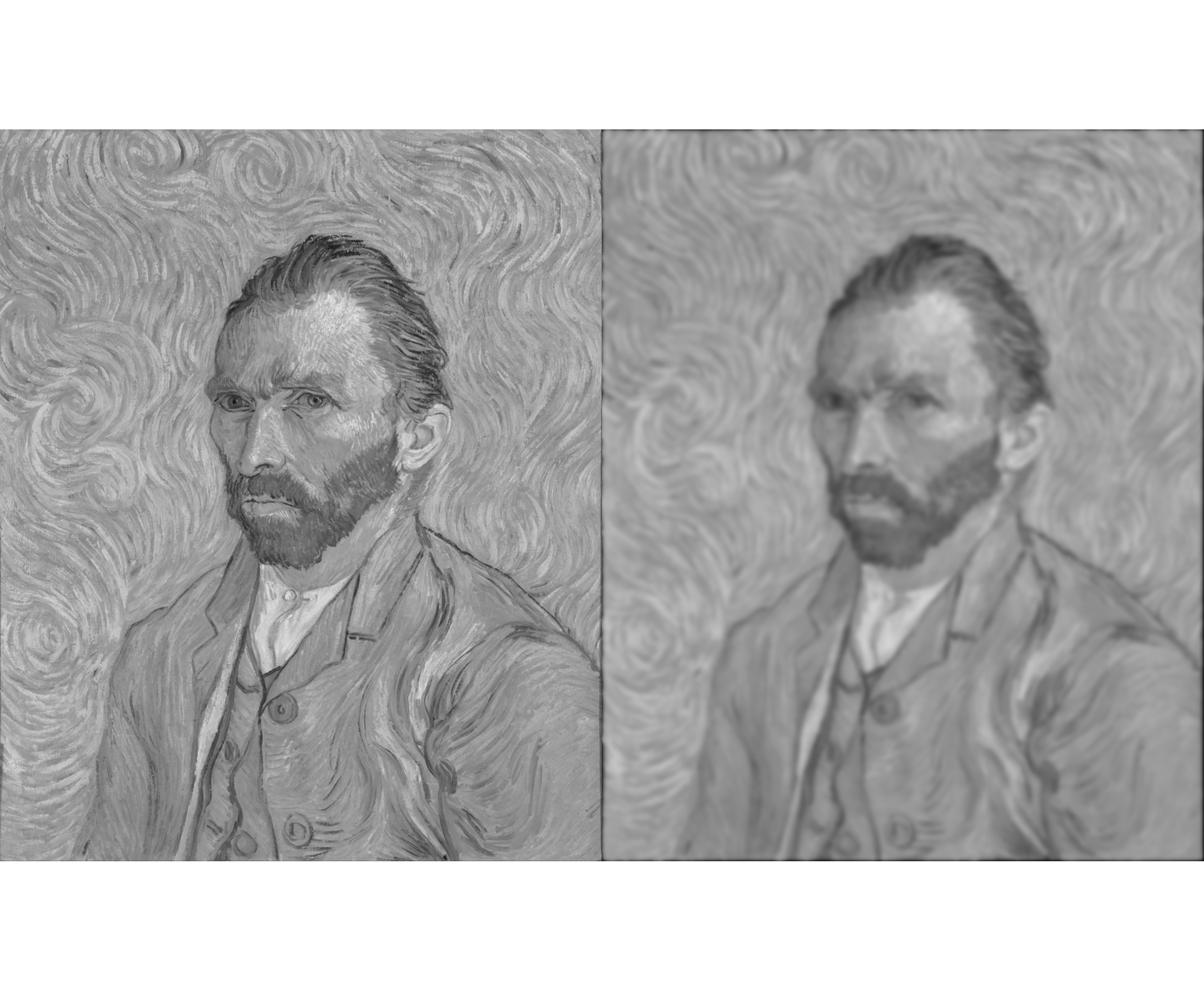
and code

im=imread("vangogh.png");
im=rgb2gray(im);
jm=uint8(anisodiff(im, 20, 100, .25, 1));

imwrite(jm,"ad-vgogh.png")

---

Back...

---

For attribution, please cite this page as:

Charters, T., "Anisotropic Diffusion example": https://blog.nexp.pt/nlineardifussion.html (06-09-2025 [15:20])

---

(cc-by-sa) Tiago Charters - tiagocharters@nexp.pt