Some mathematical notes on a polargraph

... and physics too

A V-Bot is a simple drawing machine based on two-center bipolar coordinates. Here's some web references:

The first: HECTOR
The smartest: Der Kritzler
The saddest: SADbot - the Seasonally Affected Drawing robot
The coolest: IOIO Plotter

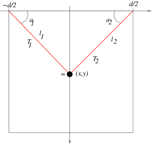
The layout of a V-Bot is quite simple, two motors at the upper vertices at a distance d, with two strings attached with lengths l1 and l2. The drawing pen rests at (x,y).

Problems to solve

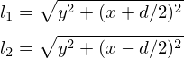
The typical math problems associated with robots are two: direct and inverse kinematics. In this particular case the inverse kinematics is easy to obtain, given the pen position obtain the lengths of the strings:

$latex2png equation$

I'm using GNU/Octave, so here's some auxiliary functions:

function retval=l1c(x,y,d)
  retval= sqrt(y.^2+(x+d/2).^2);
end

function retval=l2c(x,y,d)
  retval= sqrt(y.^2+(x-d/2).^2);
end

These equations define a map from the cartesian coordinates (x,y) to (l1,l2).

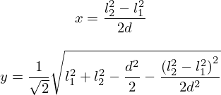
For the direct kinematics one has, with some simple algebra, $latex2png equation$

Drawing resolution

One can tackle the problem of finding the resolution in two ways. Using the Jacobian and the arc length of a curve.

The Jacobian

The Jacobian $latex2png equation$ defines the ratio of a unit area in both coordinates. That is, it controls what happens (direct kinematics) when a unit area in (l1,l2) coordinates is transformed in to (x,y) coordinates, it expands, contracts or stays the same. Values for J greater than one gives an area expansion, lower than one the area is reduced. The Jacobian controls the resolution of the drawing region.

What happens when the Jacobian is zero? In simple terms it means that the transformation breaks, i.e. one can not use the transformation between (x,y) and (l1,l2) to control the robot, and so at the points or at the lines where Jacobian is zero the robot can not be controlled (you can guess by simple inspection, with no math, what these lines/points are ;) ).

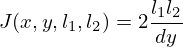
The Jacobian $latex2png equation$ is given by $latex2png equation$

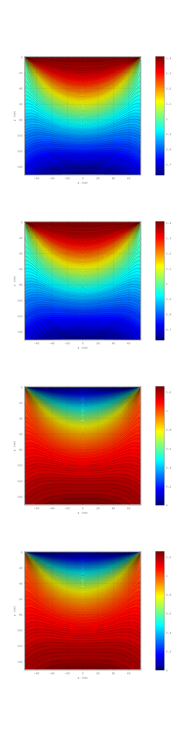
The next image shows the value of this Jacobian as a function of (x,y)

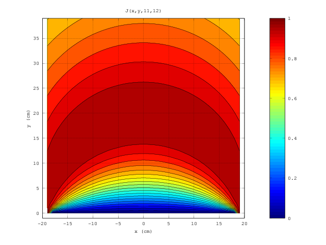
The code for the Jacobian J(x,y,l1,l2) is given by

function retval=jac(x,y,d)
  retval=2*1c(x,y,d).*l2c(x,y,d)./(d*y);
end

For the inverse kinematics the Jacobian is the reciprocal of J(x,y,l1,l2), that is 1/J(x,y,l1,l2). In this case one gets

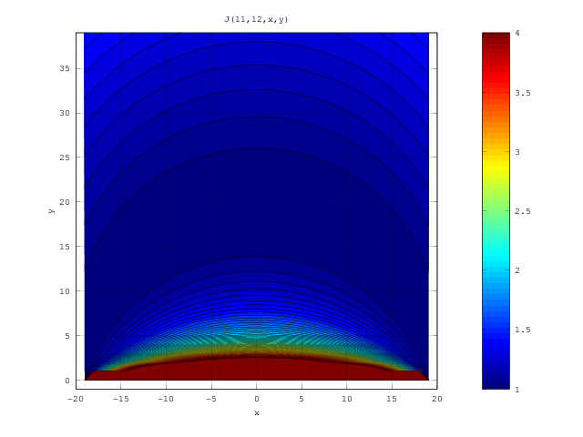
As expected (see pics) the problematic lines are l1+l2=d or simply the line y=0 for any x.

The previous plots shows the "good" areas for drawing, somewhere below the y=0 line (10cm?). Will see the same result when considering the tension on the strings (see below).

The arc length of a curve

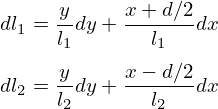
The the arc length of a curve can be used to determine the "good" plotting region for the robot. This is done by taking the first order Taylor expansion of the direct and inverse kinematics equations. This however requires some prior considerations.

Because the relation between (x,y) and (l1,l2) is non-linear any variation (x,y) will produce a non-linear variation in (l1,l2) this variation is path dependent, the propagation of the variations depends if, for example, the pen goes right and then up or by the hypotenuse to the same point on the drawing board.

$latex2png equation$ and $latex2png equation$

Here goes:

function retval=lenghtl(x,y,dx,dy,d)
  dl1=(y.*dy+(x+d/2).*dx)./l1c(x,y,d);
  dl2=(y.*dy+(x-d/2).*dx)./l2c(x,y,d);
  retval=sqrt((dl1.^2+dl2.^2)/(dx.^2+dy.^2));
end

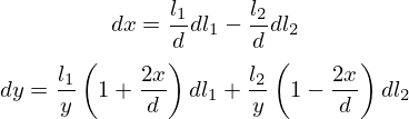
function retval=lenghtxy(x,y,dl1,dl2,d)
  dx=l1c(x,y,d)./d.*dl1 - l2c(x,y,d)./d.*dl2;
  dy=l1c(x,y,d).*(1-2*x/d)./(2*y).*dl1 + l2c(x,y,d).*(1+2*x/d)./(2*y).*dl2;
  retval=sqrt((dx.^2+dy.^2)/(dl1.^2+dl2.^2));
end

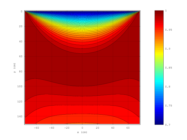
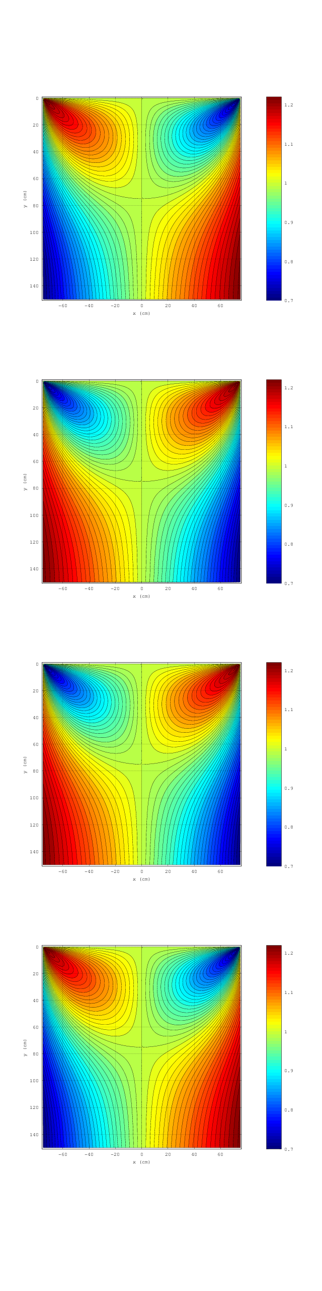
The next plot shows the ratio of unit lengths in the direct kinematics plotted in the (x,y) plane by taking the average on the 4 movements of the pen (right,0), (left,0), (0,up) and (0,down)¹.

The next plot takes the average length on 4 movements of the pen (left,up), (right,up), (left,down) and (right,down)².

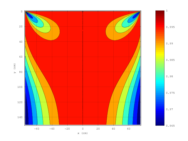
This last plot is similar to the final plot obtained by Bill Rasmussen. My point is that in this way we only account for the variation of the length of a straight segment in this coordinate transformation. Obviously the length changes after the transformation due to the non-linearity of the transformation and reflects the loss of resolution but the right way to determine the resolution is using the Jacobian.

The ends of the control lines in the above picture seem to be further away from the plotting surface than V plotters commonly seen on the internet.

That's just because the important tool to measure resolution is the Jacobian, even thought many of the V-Bot builders do not know about it ;)

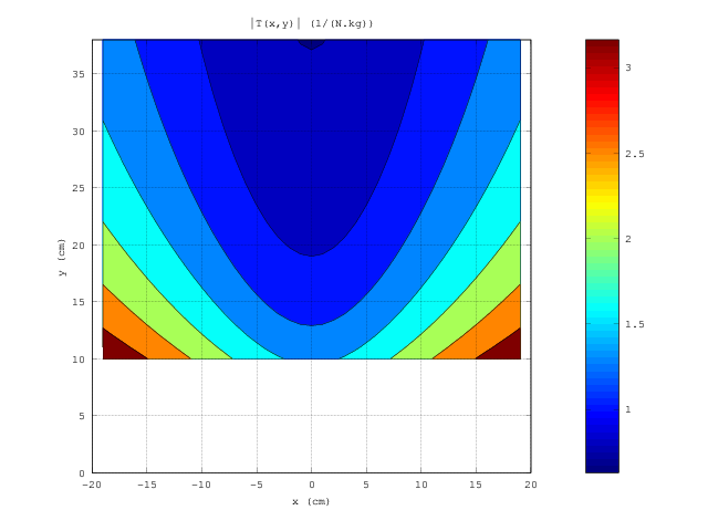
What about the tension on the strings?

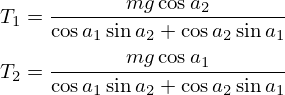
One should also take into account the tension on each string. With some trigonometry one gets

$latex2png equation$

There's only one singular configuration that one should take note, the case 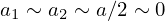$latex2png equation$ which yields $latex2png equation$

function retval=tension(x,y,d)
  m=1;
  g=1;
  l1=sqrt(y.^2+(d/2-x).^2);
  l2=sqrt(y.^2+(d/2+x).^2);
  cosa1=(d/2+x)./l1;
  cosa2=(d/2-x)./l2;
  sina1=y./l1;
  sina2=y./l2;

  T1=m*g*cosa2./(cosa1.*sina2+cosa2.*sina1);
  T2=m*g*cosa1./(cosa1.*sina2+cosa2.*sina1);
  retval=sqrt(T1.^2+T2.^2);
end

This is shown in the following plot:

Also the cases of null tension on one of the strings $latex2png equation$ , $latex2png equation$ or $latex2png equation$ , $latex2png equation$ yields, respectivly, $latex2png equation$ and $latex2png equation$ or $latex2png equation$ and $latex2png equation$ .